The sparseMVN package consists of two user-facing functions: dmvn.sparse() computes the density of a multivariate normal (MVN) distribution, and rmvn.sparse() samples from an MVN distribution. Unlike MVN functions provided by the mvtnorm and [MASS] packages, which take a dense representation of a full covariance matrix as one of the arguments, the sparseMVN functions ask for a sparse Cholesky decomposition of either the covariance or precision matrix. When the dimension of the MVN random variable is large, and the true covariance is itself sparse (i.e., the proportion of nonzero elements is small), sparseMVN offers the following advantages.

Memory use and computation time in matrix operations: A dense matrix in R stores all $M^2$ elements, even if the matrix is symmetric, and even when a small proportion of elements are nonzero. Thus, memory requirements grow quadratically with the size of the problem. Further, dense Cholesky factorization is a $\mathcal{O}\!\left(M^3\right)$ operation, while multiplication of a triangular matrix with a dense matrix, and solving dense triangular systems, are $\mathcal{O}\!\left(M^2\right)$ (Golub and Van Loan 1996). sparseMVN replies on classes from the Matrix package that compresses sparse matrices into an efficient structure for storage, and provides optimized algorithms for operations on those matrices. So, working with MVN distributions becomes more scalable when the covariance or precision matrix is actually sparse. The reasons are that only nonzero elements are stored explicitly, and redundant multiplications with zero are avoided.
Avoiding explicit inversion of a precision matrix. In many applications (e.g., sampling from a Laplace approximation), the user starts with a sparse precision matrix rather than a covariance. Using extant MVN functions in R requires the user to explicitly invert the precision matrix, which itself can be an expensive step, with no guarantee of sparsity afterward. But this inversion step is not mathematically necessary; computation of MVN densities and random variates can be done just as easily and directly with the precision matrix. At the user’s option, sparseMVN accepts a factor of either a sparse covariance or precision matrix.
Multiple-use Cholesky factorization. MVN computation involves computing the Cholesky factor of the matrix (either covariance or precision). Most MVN functions do this internally (so the user does not have to worry about it) every time the function is called (which is wasteful if the matrix does not change from call to call). sparseMVN requires the user to perform this step separately with Matrix::Cholesky(). While this feature does impose one additional step on the user, it also allows the user to reuse the same factor when possible.

Background

Let $x\in\mathbb{R}^{M}$ be a realization of random variable $X\sim\mathbf{MVN}\!\left(\mu,\Sigma\right)$, where $\mu\in\mathbb{R}^{M}$ is a vector, $\Sigma\in\mathbb{R}^{M\times M}$ is a positive-definite covariance matrix, and $\Sigma^{-1}\in\mathbb{R}^{M\times M}$ is a positive-definite precision matrix.

The log probability density of $x$ is

\[\begin{aligned} \log f(x)&=-\frac{1}{2}\left(M \log (2\pi) + \log|\Sigma| +z^\top z\right),\quad\text{where}~z^\top z=\left(x-\mu\right)^\top\Sigma^{-1}\left(x-\mu\right) \end{aligned}\]

MVN density computation and random number generation

The two computationally intensive steps in evaluating $\log f(x)$ are computing $\log|\Sigma|$, and $z^\top z$, without explicitly inverting $\Sigma$ or repeating mathematical operations. But once we have $z$, computing the dot product $z^\top z$ is cheap. How to perform these steps efficiently in practice depends on whether the covariance matrix $\Sigma$, or the precision matrix $\Sigma^{-1}$ is available. For both cases, we start by finding a lower triangular matrix root: $\Sigma=LL^\top$ or $\Sigma^{-1}=\Lambda\Lambda^\top$. Since $\Sigma$ and $\Sigma^{-1}$ are positive definite, we will use the Cholesky decomposition, which is the unique matrix root with all positive elements on the diagonal.

With the Cholesky decomposition in hand, we compute the log determinant of $\Sigma$ by adding the logs of the diagonal elements of the factors. \[\begin{aligned} \label{eq:logDet} \log|\Sigma|= \begin{cases} \phantom{-}2\sum_{m=1}^M\log L_{mm}&\text{ when $\Sigma$ is given}\\ -2\sum_{m=1}^M\log \Lambda_{mm}&\text{ when $\Sigma^{-1}$ is given} \end{cases}\end{aligned}\]

Having already computed the triangular matrix roots also speeds up the computation of $z^\top z$. If $\Sigma^{-1}$ is given, $z=\Lambda^\top(x-\mu)$ can be computed efficiently as the product of an upper triangular matrix and a vector. When $\Sigma$ is given, we find $z$ by solving the lower triangular system $Lz=x-\mu$. The subsequent $z^\top z$ computation is trivially fast.

The algorithm for simulating $X\sim\mathbf{MVN}\!\left(\mu,\Sigma\right)$ also depends on whether $\Sigma$ or $\Sigma^{-1}$ is given. As above, we start by computing the Cholesky decomposition of the given covariance or precision matrix. Define a random variable $Z\sim\mathbf{MVN}\!\left(0,I_M\right)$, and generate a realization $z$ as a vector of $M$ samples from a standard normal distribution. If $\Sigma$ is given, then evaluate $x=Lz+\mu$. If $\Sigma^{-1}$ is given, then solve for $x$ in the triangular linear system $\Lambda^\top\left(x-\mu\right)=z$. The resulting $x$ is a sample from $\mathbf{MVN}\!\left(\mu,\Sigma\right)$. The following shows that this approach is correct:

\[\begin{aligned} \mathbf{E}\!\left(X\right)&=\mathbf{E}\!\left(LZ+\mu\right)=\mathbf{E}\!\left(\Lambda^\top Z+\mu\right)=\mu\\ \mathbf{cov}\!\left(X\right)&= \mathbf{cov}\!\left(LZ+\mu\right)=\mathbf{E}\!\left(LZZ^\top L^\top\right)=LL^\top=\Sigma\\ \mathbf{cov}\!\left(X\right)&=\mathbf{cov}\!\left((\Lambda^\top)^{-1}Z+\mu\right)=\mathbf{E}\!\left((\Lambda^\top)^{-1}ZZ^\top\Lambda^{-1}\right) =(\Lambda^\top)^{-1}\Lambda^{-1}=(\Lambda\Lambda^\top)^{-1}=\Sigma \end{aligned}\]

These algorithms apply when the covariance/precision matrix is either sparse or dense. When the matrix is dense, the computational complexity is $\mathcal{O}\!\left(M^3\right)$ for a Cholesky decomposition, and $\mathcal{O}\!\left(M^2\right)$ for either solving the triangular linear system or multiplying a triangular matrix by another matrix (Golub and Van Loan 1996). Thus, the computational cost grows cubically with $M$ before the decomposition step, and quadratically if the decomposition has already been completed. Additionally, the storage requirement for $\Sigma$ (or $\Sigma^{-1}$) grows quadratically with $M$.

Sparse matrices in R

The Matrix package (Bates and Maechler 2017) defines various classes for storing sparse matrices in compressed formats. The most important class for our purposes is dsCMatrix, which defines a symmetric matrix, with numeric (double precision) elements, in a column-compressed format. Three vectors define the underlying matrix: the unique nonzero values (just one triangle is needed), the indices in the value vector for the first value in each column, and the indices of the rows in which each value is located. The storage requirements for a sparse $M\times M$ symmetric matrix with $V$ unique nonzero elements in one triangle are for $V$ double precision numbers, $V+M+1$ integers, and some metadata. In contrast, a dense representation of the same matrix stores $M^2$ double precision values, regardless of symmetry and the number of zeros. If $V$ grows more slowly than $M^2$, the matrix becomes increasingly sparse (a smaller percentage of elements are nonzero), with greater efficiency gains from storing the matrix in a compressed sparse format.

To illustrate how sparse matrices require less memory resources when compressed than when stored densely, consider the following example, which borrows heavily from the vignette of the sparseHessianFD package.

Suppose we have a dataset of $N$ households, each with $T$ opportunities to purchase a particular product. Let $y_i$ be the number of times household $i$ purchases the product, out of the $T$ purchase opportunities, and let $p_i$ be the probability of purchase. The heterogeneous parameter $p_i$ is the same for all $T$ opportunities, so $y_i$ is a binomial random variable.

Let $\beta_i\in\mathbb{R}^{k}$ be a heterogeneous coefficient vector that is specific to household $i$, such that $\beta_i=(\beta_{i1},\dotsc,\beta_{ik})$. Similarly, $w_i\in\mathbb{R}^{k}$ is a vector of household-specific covariates. Define each $p_i$ such that the log odds of $p_i$ is a linear function of $\beta_i$ and $w_i$, but does not depend directly on $\beta_j$ and $w_j$ for another household $j\neq i$: \[\begin{aligned} p_i=\frac{\exp(w_i'\beta_i)}{1+\exp(w_i'\beta_i)},~i=1,\dots, N\end{aligned}\]

The coefficient vectors $\beta_i$ are distributed across the population of households following a MVN distribution with mean $\mu\in\mathbb{R}^{k}$ and covariance $\mathbf{A}\in\mathbb{R}^{k\times k}$. Assume that we know $\mathbf{A}$, but not $\mu$, so we place a multivariate normal prior on $\mu$, with mean $0$ and covariance $\mathbf{\Omega}\in\mathbb{R}^{k\times k}$. Thus, the parameter vector $x\in\mathbb{R}^{(N+1)k}$ consists of the $Nk$ elements in the $N$ $\beta_i$ vectors, and the $k$ elements in $\mu$.

The log posterior density, ignoring any normalization constants, is \[\begin{aligned} \label{eq:LPD} \log \pi(\beta_{1:N},\mu|\mathbf{Y}, \mathbf{W}, \mathbf{A},\mathbf{\Omega})=\sum_{i=1}^N\left(p_i^{y_i}(1-p_i)^{T-y_i} -\frac{1}{2}\left(\beta_i-\mu\right)^\top\mathbf{A}^{-1}\left(\beta_i-\mu\right)\right) -\frac{1}{2}\mu^\top\mathbf{\Omega}^{-1}\mu\end{aligned}\]

Because one element of $\beta_i$ can be correlated with another element of $\beta_i$ (for the same unit), we allow for the cross-partials between elements of $\beta_i$ for any $i$ to be nonzero. Also, because the mean of each $\beta_i$ depends on $\mu$, the cross-partials between $\mu$ and any $\beta_i$ can be nonzero. However, since the uild$\beta_i$ and $\beta_j$ are independent samples, and the $y_i$ are conditionally independent, the cross-partial derivatives between an element of $\beta_i$ and any element of any $\beta_j$ for $j\neq i$, must be zero. When $N$ is much greater than $k$, there will be many more zero cross-partial derivatives than nonzero, and the Hessian of the log posterior density will be sparse.

The sparsity pattern depends on how the variables are ordered. One such ordering is to group all of the coefficients in the $\beta_i$ for each unit together, and place $\mu$ at the end. \[\begin{aligned} \beta_{11},\dotsc,\beta_{1k},\beta_{21},\dotsc,\beta_{2k},~\dotsc~,\beta_{N1},\dotsc,\beta_{Nk},\mu_1,\dotsc,\mu_k\end{aligned}\] In this case, the Hessian has a “block-arrow” pattern. This figure illustrates this pattern for $N=5$ and $k=2$ (12 total variables).

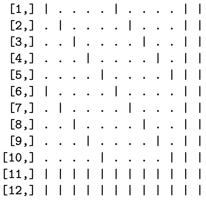
Block arrow (left) and banded (right) sparsity patterns

Another possibility is to group coefficients for each covariate together. \[\begin{aligned} \beta_{11},\dotsc,\beta_{N1},\beta_{12},\dotsc,\beta_{N2},~\dotsc~,\beta_{1k},\dotsc,\beta_{Nk},\mu_1,\dotsc,\mu_k\end{aligned}\] Now the Hessian has an "banded" sparsity pattern:

In both cases, the number of nonzeros is the same. There are 144 elements in this symmetric matrix. If the matrix is stored in the standard base R dense format, memory is reserved for all 144 values, even though only 64 values are nonzero, and only 38 values are unique. For larger matrices, the reduction in memory requirements by storing the matrix in a sparse format can be substantial. If $N=1,000$ and $k=2$, then $M=$ 2,002, with more than $4$ million elements in the Hessian. However, only 12,004 of those elements are nonzero, with 7,003 unique values in the lower triangle. The dense matrix requires 30.6 Mb of RAM, while a sparse symmetric dsCMatrix matrix requires only 91.6 Kb.

This example is relevant because, when evaluated at the posterior mode, the Hessian matrix of the log posterior is the MVN precision matrix $\Sigma^{-1}$ of a MVN approximation to the posterior distribution of $\left(\beta_{1:N},\mu\right)$. If we were to simulate from this MVN using , or evaluate MVN densities using , we would need to invert $\Sigma^{-1}$ to $\Sigma$ first, and store it as a dense matrix. Internally, and invoke dense linear algebra routines, including matrix factorization.

Using the sparseMVN package

The signatures of the key sparseMVN functions are

rmvn.sparse(n, mu, CH, prec=TRUE, log=TRUE)
dmvn.sparse(x, mu, CH, prec=TRUE, log=TRUE)

rmvn.sparse() returns a matrix $x$ with $n$ rows and length(mu) columns. dmvn.sparse() returns a vector of length n: densities if log=FALSE , and log densities if log=TRUE.

x	A numeric matrix. Each row is an MVN sample.
mu	A numeric vector. The mean of the MVN random variable.
CH	Either a dCHMsimpl or dCHMsuper object representing the Cholesky decomposition of the covariance/precision matrix.
prec	Logical value that identifies CH as the Cholesky decomposition of either a covariance ($\Sigma$, ) or precision($\Sigma^{-1}$, ) matrix.
n	Number of random samples to be generated.
log	If `log=TRUE`, the log density is returned.

[Table 1: Arguments to dmvn.sparse() and rmvn.sparse()]

dmvn.sparse() and rmvn.sparse() require the user to compute the Cholesky decomposition CH beforehand, but this needs to be done only once (as long as $\Sigma$ or $\Sigma^{-1}$ does not change). CH should be computed using Cholesky(), whose first argument is a sparse symmetric matrix stored as a dsCMatrix object. As far as we know, there is no particular need to deviate from the defaults of the remaining arguments. If Cholesky() uses a fill-reducing permutation to compute CH , the sparseMVN functions will handle that directly, with no additional user intervention required. The chol() function in base R should not be used.

An example

Suppose we want to generate samples from an MVN approximation to the posterior distribution of our example model from Section 1.2. sparseMVN includes functions to simulate data and compute the log posterior density, gradient and Hessian for the binary choice example model. The trustOptim package provides a nonlinear optimizer that estimates the curvature of the objective function using a sparse Hessian.

The calls to trust.optim() return the posterior mode, and the Hessian evaluated at the mode. These results serve as the mean and the negative precision of the MVN approximation to the posterior distribution of the model.

We can then sample from the posterior using an MVN approximation, and compute the MVN log density for each sample.

samples <- sparseMVN::rmvn.sparse(R, pm, CH, prec=TRUE)
logf <- sparseMVN::dmvn.sparse(samples, pm, CH, prec=TRUE)

The ability to accept a precision matrix, rather than having to invert it to a covariance matrix, is a valuable feature of sparseMVN. This is because the inverse of a sparse matrix is not necessarily sparse. In the following chunk, we invert the Hessian, and drop zero values to maintain any remaining sparseness. Note that there are 10,404 total elements in the Hessian.

Matrix::nnzero(H)
Hinv <- Matrix::drop0(solve(H))
Matrix::nnzero(Hinv)

Nevertheless, we should check that the log densities from dmvn.sparse() correspond to those that we would get from dmvnorm().

logf_dense <- mvtnorm::dmvnorm(samples, pm, as.matrix(Hinv), log=TRUE)
all.equal(logf, logf_dense)

Performance

In this section we show the efficiency gains from sparseMVN by comparing the run times between rmvn.sparse() and rmvnorm(), and between dmvn.sparse() and mvtnorm::dmvnorm. In these tests, we construct covariance/precision matrices with the same structure as the Hessian of the log posterior density of the example model in Section 2.1. Parameters are ordered such that the matrix has a block-arrow pattern (Figure @ref(fig:sparse-patterns), left).

The following table summarizes the case conditions. $N$ and $k$ refer, respectively, to the number of blocks in the block-arrow structure (analogous to heterogeneous units in the binary choice example), and the size of each block. The total number of variables is $M=(N+1)k$, and the total number of elements in the matrix is $M^2$. The three rightmost columns present the number of nonzeros in the full matrix and lower triangle, and the sparsity (proportion of matrix elements that are nonzero. The size and sparsity of the test matrices vary through manipulation of the number of blocks ($N$), the size of each block ($k$), and the number of rows/columns in the margin (also $k$). Each test matrix has $(N+1)k$ rows and columns.

Cases for the timing comparison.
				nonzeros
k	N	variables	elements	full	lower tri	sparsity
2	10	22	484	124	73	0.256
2	20	42	1,764	244	143	0.138
2	50	102	10,404	604	353	0.058
2	100	202	40,804	1,204	703	0.030
2	200	402	161,604	2,404	1,403	0.015
2	300	602	362,404	3,604	2,103	0.010
2	400	802	643,204	4,804	2,803	0.007
2	500	1,002	1,004,004	6,004	3,503	0.006
4	10	44	1,936	496	270	0.256
4	20	84	7,056	976	530	0.138
4	50	204	41,616	2,416	1,310	0.058
4	100	404	163,216	4,816	2,610	0.030
4	200	804	646,416	9,616	5,210	0.015
4	300	1,204	1,449,616	14,416	7,810	0.010
4	400	1,604	2,572,816	19,216	10,410	0.007
4	500	2,004	4,016,016	24,016	13,010	0.006

Figure @ref(fig:densRand) compares mean run times to compute 1,000 MVN densities, and generate 1,000 MVN samples, using rmvn.sparse() and dmvn.sparse() from sparseMVN, and dmvnorm() and rmvnorm() in sparseMVN. Times were collected over 200 replications on a 2013-vintage Mac Pro with a 12-core 2.7 GHz Intel Xeon E5 processor and 64 GB of RAM. The times for mvtnorm are faster than sparseMVN for low dimensional cases ($N\leq 50$), but grow quadratically in the number of variables. This is because the number of elements stored in a dense covariance matrix grows quadratically with the number of variables. In this example, storage and computation requirements for the sparse matrix grow linearly with the number of variables, so the sparseMVN run times grow linearly as well (Braun and Damien 2016). The comparative advantage of sparseMVN increases with the sparsity of the covariance matrix.[^5]

Mean computation time for simulating 1,000 MVN samples, and computing 1,000 MVN densities, averaged over 200 replications. Densities were computed using [dmvnorm] and dmvn.sparse(), while random samples were generated using rmvnorm() and rmvn.sparse().

The sparseMVN functions always require a sparse Cholesky decomposition of the covariance or precision matrix, and the mvtnorm functions require a dense precision matrix to be inverted into a dense covariance matrix. Figure @ref(fig:cholSolve) compares the computation times of these preparatory steps. There are three cases to consider: inverting a dense matrix using solve(), decomposing a sparse matrix using Matrix::Cholesky(), and decomposing a dense matrix using chol(). Applying chol() to a dense matrix is not a required operation in advance of calling dmvnorm() or rmvnorm(), but those functions will invoke some kind of decomposition internally. We include it in our comparison because it comprises a substantial part of the computation time. The decomposition and inversion operations on the dense matrices grow cubically as the size of the matrix increases. The sparse Cholesky decomposition time is negligible. For example, the mean run time for the $N=500$, $k=4$ case is about 0.39 ms.

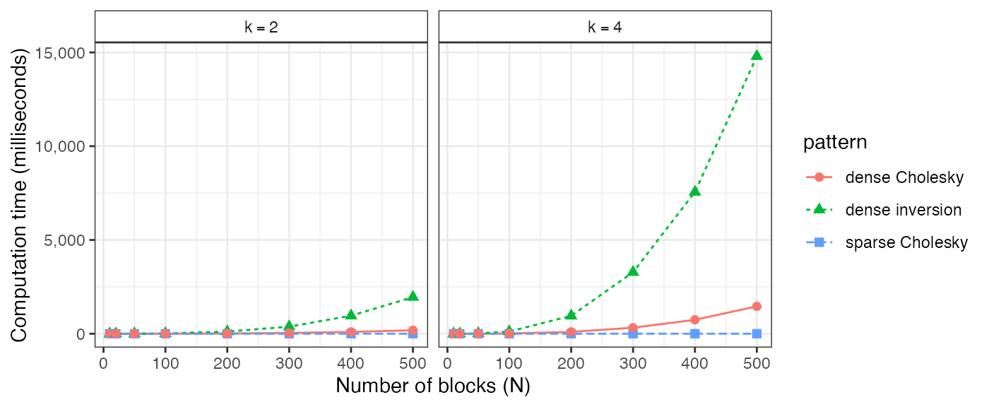
Computation time for Cholesky decomposition of sparse and dense matrices, and inversion of dense matrices.

References

Bates, Douglas, and Martin Maechler. 2017. : Sparse and Dense Matrix Classes and Methods. https://CRAN.R-project.org/package=Matrix.

Braun, Michael, and Paul Damien. 2016. “Scalable Rejection Sampling for Bayesian Hierarchical Models.” Marketing Science 35 (3): 427–44. https://doi.org/10.1287/mksc.2014.0901.

Golub, Gene H, and Charles F Van Loan. 1996. Matrix Computations. 3rd ed. Johns Hopkins University Press.

The sparseMVN package

Michael Braun, Cox School of Business, Southern Methodist University